


qp.TrotterVibronic
- class TrotterVibronic(evolution_time, num_trotter_steps, hamiltonian, *, cache_wires=(), coefficient_wires=(), electronic_wires, phase_gradient_wires, vib_wires, work_wires=(), aqft_order=None, branch_probs=None)[source]
Bases:
Operator2Second-order Trotter circuit for vibronic Hamiltonian simulation using phase-gradient arithmetic.
This template realizes \(U \approx e^{-iHt}\) for a vibronic Hamiltonian, using the phase-gradient arithmetic construction of Motlagh et al, arXiv:2411.13669,
\[H = \sum_{i=0}^{F-1} H_i + H_{\text{kin}}, \qquad H_i = V_i D_i(Q) V_i^\dagger, \qquad H_{\text{kin}} = \sum_r t_r P_r^2 .\]See also
- Parameters:
evolution_time (float) – time \(t\) for which to evolve under the vibronic Hamiltonian.
num_trotter_steps (int) – number of second-order Trotter steps to use.
hamiltonian (
pennylane.VibronicHamiltonian) – Apennylane.VibronicHamiltonianinstance whose arguments areconstant,linear,quadraticandkinetic. The expected shapes areconstant: (F, N, N),linear: (F, N, N, M),quadratic: (F, N, N, M, M)andkinetic: (N, N, M, M), whereFis the number of position fragments,Nthe number of electronic states andMthe number of vibrational modes.Nmust be a power of 2, and the fragments must follow the “XOR” scheme described in the Implementation Details section. See the documentation forpennylane.VibronicHamiltonianfor more information.electronic_wires (WiresLike) – the \(n\) electronic-state wires.
vib_wires (WiresLike) – the \(M \cdot k\) vibrational-mode wires, provided as a single flattened register. Internally these are reshaped into
Mregisters ofkwires, one per mode, vianp.array(vib_wires).reshape(M, -1).phase_gradient_wires (WiresLike) – at least \(b\) wires holding the phase-gradient resource state, assumed to be prepared upfront. Only the first \(b\) wires are used.
coefficient_wires (WiresLike) – the \(b\) wires of the Hamiltonian-coefficient register. If omitted (default), they are dynamically allocated in the decomposition, with \(b\) equal to
len(phase_gradient_wires).cache_wires (WiresLike) – the \(2k\) cache wires for squared/multiplied mode registers. If omitted (default), they are dynamically allocated in the decomposition.
work_wires (WiresLike) – the \(\max(n-1, b+1, 2k+2)\) work wires for data loading and arithmetic. If omitted (default), they are dynamically allocated in the decomposition.
aqft_order (int) – approximation order of the
AQFTused to transform between position and momentum space. IfNone(default), no approximation is made (aqft_order = k - 1).branch_probs (dict[str, float]) – probabilities for the fragment terms to be applied rather than skipped for vanishing coefficients, used as resource hints. See note below for details.
Example
Let’s first create a
pennylane.VibronicHamiltonianwith dummy data.import numpy as np import pennylane as qp n_states, n_modes, k, b = 2, 1, 2, 3 n = int(np.ceil(np.log2(n_states))) # A single diagonal position fragment with non-zero constant/linear coefficients, and a # diagonal kinetic fragment. constant = np.zeros((1, n_states, n_states)) constant[0, 0, 0], constant[0, 1, 1] = 0.4, -0.4 linear = np.zeros((1, n_states, n_states, n_modes)) linear[0, 0, 0, 0], linear[0, 1, 1, 0] = 0.2, -0.2 hamiltonian = qp.VibronicHamiltonian( constant=constant, linear=linear, quadratic=np.zeros((1, n_states, n_states, n_modes, n_modes)), kinetic=np.einsum( "ab,cd->abcd", np.eye(n_states), np.diag(0.3 * np.ones(n_modes)) ), )
With this, we can setup a simple circuit that includes
TrotterVibronic.wires = qp.registers({ "electronic": n, "vib_wires": n_modes * k, "cache": 2 * k, "coefficients": b, "phase_gradient": b, "work": max(n - 1, b + 1, 2 * k + 2), }) all_wires = qp.wires.Wires.all_wires(list(wires.values())) # decompose by one step to see the top-level sub-templates @qp.transforms._tape_decompose(max_expansion=1, gate_set=qp.gate_sets.ALL_OPS | {qp.PhaseGradientStatePrep}) @qp.qnode(qp.device("default.qubit", wires=all_wires)) def circuit(): qp.PhaseGradientStatePrep(wires["phase_gradient"]) qp.TrotterVibronic( evolution_time=1.0, num_trotter_steps=1, hamiltonian=hamiltonian, electronic_wires=wires["electronic"], vib_wires=wires["vib_wires"], cache_wires=wires["cache"], coefficient_wires=wires["coefficients"], phase_gradient_wires=wires["phase_gradient"], work_wires=wires["work"], aqft_order=1, ) return qp.probs(wires=wires["electronic"])
>>> qp.specs(circuit)().resources.quantum_operations
{'PhaseGradientStatePrep': 1, 'QROM': 6, 'SemiAdder': 4, 'PauliX': 28, 'C(MultiX)': 8, 'MultiControlledX': 16, 'TemporaryAND': 10, 'CNOT': 48, 'Adjoint(TemporaryAND)': 10, 'AQFT': 1, 'MultiX': 2, 'SignedOutSquare': 1, 'OutMultiplier': 1, 'Adjoint(SignedOutSquare)': 1, 'Adjoint(AQFT)': 1}
Note
The keys of
branch_probsare"constant","linear","quadratic","bilinear"and"kinetic". The probabilities are attached as"branch-prob"hints viahint()to the conditionals that skip the respective terms, and thus only expect resource accounting but not the circuit itself. In addition, they weight the gate counts of the terms in the resources of the decomposition rule, and thus affect the weight of this rule in the graph-based decomposition system.If
branch_probs=None(default), the probablities are computed fromhamiltonianandevolution_timeif both are concrete, and omitted otherwise.Providing
branch_probsreplaces the probabilities computed fromhamiltonianandevolution_timeentirely, rather than updating them. Terms missing frombranch_probsare left unhinted and counted at every visit.Available decompositions
Resources are general, for \(F\) position fragments, \(M\) modes with \(k\) wires each, \(n\) electronic wires, \(b\) coefficient and phase gradient wires, and \(r\) =
num_trotter_steps. Each circuit shows one example of the rule. Use a rule when decomposing withqp.decompose:qp.decompose(gate_set=..., fixed_decomps={qp.TrotterVibronic: "<name>"})
vibronic_trotter_steps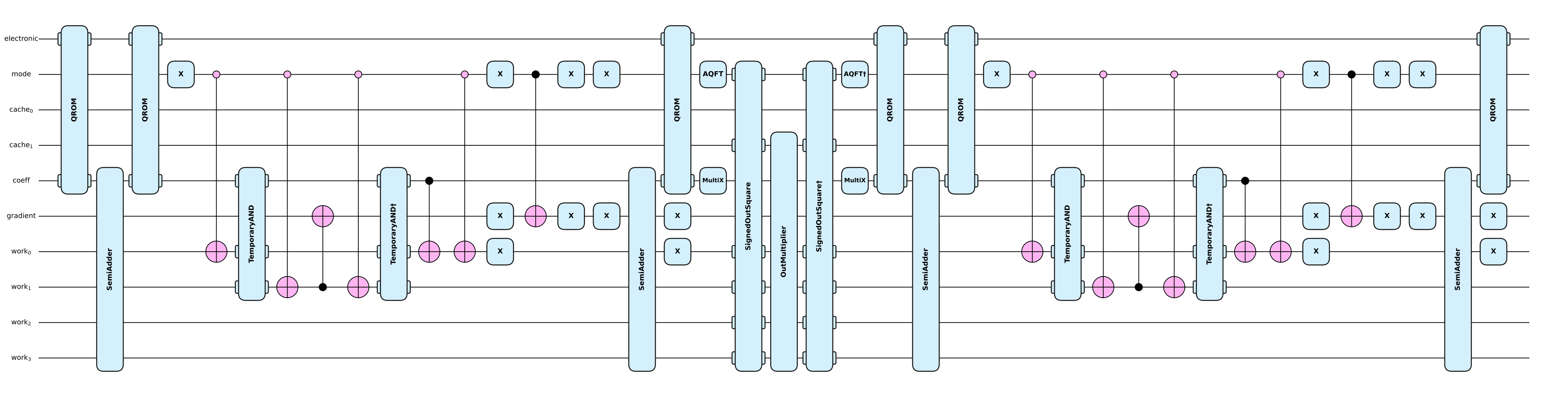
Example: \(F=1\), \(M=1\), \(k=1\), \(n=1\), \(b=1\), \(r=1\)
Gate
Count
Example
\(2P\)
0
\(2P(n-1) + 3Pk(M(2b-k) + 4K(b-k))\)
6
\(P(M + K)(2b + 8)\)
20
Xwith 1 control on \(|0\rangle\)\(4Pk(M + 2K)\)
8
MultiXwith 1 control on \(|0\rangle\)\(2Pk(M + 2K)\,[b > 1]\)
0
\(\tfrac{Pk}{2}(M(2b-k+1) + 2K(2b-2k+1))\)
2
\(\tfrac{Pk}{2}(M(2b-k+1) + 2K(2b-2k+1))\)
2
\(P(2 + 2M + K)\)
6
\(P(1 + M + K)\)
4
\(PM + rM\)
1
\(PM + rM\)
1
\(PM + rM\)
1
\(PK\)
0
\(PK\)
0
\(2rM\)
2
\(rM\)
1
\(rM\)
1
where \(P = 2Fr\) position-fragment visits and \(K = M(M-1)/2\) mode pairs, and \([b > 1]\) is 1 if \(b > 1\) and 0 otherwise. All counts are upper bounds: terms with zero coefficients are skipped, and the
HadamardandCNOTcounts also depend on each fragment’s electronic diagonalization. The counts of the gates from the half-signed multipliers assume \(k \leq b\), and \(2k \leq b\) if \(K > 0\)Register Sizes
With \(N\) electronic states (\(n = \lceil\log_2(N)\rceil\) qubits), \(M\) vibrational modes (\(k\) qubits each), and \(b\)-qubit coefficient and phase-gradient registers, the wire registers should have the following sizes:
Argument
Expected size
Physical meaning / information content
electronic_wires\(n\)
electronic state
vib_wires\(M \cdot k\)
positions of all vibrational modes (signed), flattened
cache_wires\(2k\)
cached squares/products of modes (signed/unsigned)
coefficient_wires\(b\)
Hamiltonian coefficients (unsigned); optional, dynamically allocated if omitted
phase_gradient_wires\(\ge b\)
phase-gradient state (unsigned)
work_wires\(\max(n-1, b+1, 2k+2)\)
data-loading/arithmetic scratch
Implementation Details
This section shows how the dense
pennylane.VibronicHamiltonianis turned into gates, making every phase prefactor explicit, following Motlagh et al, arXiv:2411.13669 (see also this PennyLane demo for a from-scratch, step-by-step implementation). The mode positions \(Q_r\) and momenta \(P_r\) are the signed (two’s-complement) integers on the mode sub-registers ofvib_wires, and \(a\) labels anelectronic_wiresbasis state. Operator products below use the standard convention that the rightmost factor is applied first.The Hamiltonian is a sum of \(F\) position fragments and one kinetic fragment,
\[H = \sum_{i=0}^{F-1} H_i + H_{\text{kin}}, \qquad H_i = V_i D_i(Q) V_i^\dagger, \qquad H_{\text{kin}} = \sum_r t_r P_r^2 .\]Here \(V_i\) (step 3) rotates into a fragment-specific electronic eigenbasis, and \(D_i(Q)\) is the diagonal generator on
electronic_wires,\[D_i(Q) = \sum_a \theta_{i,a}(Q) |a\rangle\langle a|,\]whose entries for electronic state \(a\) are degree-2 polynomials in the mode positions,
\[\theta_{i,a}(Q) = c_a + \sum_r l_{a,r} Q_r + \sum_r q_{a,r} Q_r^2 + \sum_{r<s} \beta_{a,rs} Q_r Q_s .\]The entries \(c, l, q, \beta\) are the diagonalized
constant/linear/quadratictensors of theVibronicHamiltonianand \(t_r\) the diagonal of itskinetictensor. Thequadratictensor packs both \(q_{a,r}\) (diagonal,[..., r, r]) and \(\beta_{a,rs}\) (read once from the entry with \(r < s\)). The mirror entry \((s, r)\) is ignored, so put the full weight on \(r < s\). Splitting it evenly between the two would drop half.The Hamiltonian must follow the “XOR” fragmentation scheme of the reference above: position fragment \(i\) may only populate the electronic matrix elements at index pairs \((j, i \oplus j)\) (bitwise XOR), for \(i = 0, \dots, F-1\). This is what lets \(V_i\) (step 3) be the fixed single-Hadamard/CNOT circuit derived from the key \((0, i)\). A Hamiltonian with a different fragment structure will silently produce an incorrect circuit. \(N\) itself must be a power of 2, since \(V_i\) is only guaranteed orthogonal when it spans the full \(2^n\)-dimensional electronic space. See the demo’s fragmentation and diagonalization section for the general (non-XOR) construction of \(V_i\).
1. Second-order Trotter. With \(n_T =\)
num_trotter_stepsand \(\Delta t = t/n_T\), \(e^{-iHt}\) is approximated by \(n_T\) repetitions of the symmetric step\[S_2(\Delta t) = \Big(\prod_{i=0}^{F-1} e^{-i H_i \Delta t/2}\Big) e^{-i H_{\text{kin}} \Delta t} \Big(\prod_{i=F-1}^{0} e^{-i H_i \Delta t/2}\Big),\]so each position fragment is visited twice per step at \(\tau = \Delta t/2\) and the kinetic fragment once at \(\Delta t\). See the demo’s assembling the Trotter step section for the fragment loop this unrolls into.
2. Phase-gradient arithmetic. Each fragment is diagonal, so evolving it reduces to imprinting a phase per basis state with the phase-gradient trick: the
phase_gradient_wiresare required to hold\[|\nabla n\rangle = \tfrac{1}{\sqrt{2^b}}\sum_{j=0}^{2^b-1} e^{-2\pi i j/2^b}|j\rangle, \qquad \text{ADD}(m)|\nabla n\rangle = e^{+2\pi i m/2^b}|\nabla n\rangle .\]A phase \(\tau\,\theta_{i,a}\) is imprinted by loading its \(b\)-bit fixed-point encoding \(m\) into
coefficient_wiresand adding it intophase_gradient_wireswith aSemiAdder:coefficient : ─|m⟩─╭SemiAdder─|m⟩─┤ |∇n⟩ : ─────╰SemiAdder─────┤ e^{+2πi m/2^b}|∇n⟩The sign of the ADD identity is positive, so coefficients are negated before encoding, \(m = \text{encode}(-\tau\theta_{i,a})\), giving the target \(e^{-i\tau\theta}\). Rounding to \(b\) bits (mod \(2\pi\)) is a discretization error on top of the Trotter truncation.
3. Electronic diagonalization. Each position fragment is diagonalized by a Clifford \(V_i\) (Fig. 2 of the reference),
\[e^{-i H_i \tau} = V_i e^{-i D_i(Q)\tau} V_i^\dagger, \qquad V_i = \Big(\prod_{j \ne c} \text{CNOT}_{c \to j}\Big) H_c, \quad V_0 = I .\]Here \(c\) is the least-significant set bit of \(i\), and the product runs over its other set bits \(j\). For \(i = 3\) on two
electronic_wires:electronic[0]: ──────╭X─┤ electronic[1]: ──H───╰●─┤
4. Position fragment. Each monomial of \(\theta_{i,a}(Q)\) follows the same pattern: a
QROMcontrolled onelectronic_wiresloads its coefficient intocoefficient_wires(differentially, i.e. only the change from the previous term), an arithmetic block writes the monomial’s phase intophase_gradient_wiresas in step 2, and a finalQROMunloads the last coefficient back to \(|0\rangle\):electronic : ─╭QROM─────────────╭QROM─┤ coefficient : ─╰QROM─╭arithmetic─╰QROM─┤ |∇n⟩ : ───────╰arithmetic───────┤ e^{-iτ θ}The arithmetic block per monomial (skipped when the coefficient vanishes):
\(c_a\) –
SemiAdder.\(l_{a,r} Q_r\) – a half-signed multiply of the (unsigned) coefficient by the signed \(Q_r\).
\(q_{a,r} Q_r^2\) –
SignedOutSquarethen a plainOutMultiplier.\(\beta_{a,rs} Q_r Q_s\) –
SignedOutMultiplierthen the same half-signed multiply as the linear term.
The half-signed multiply uses the controlled add/subtract decomposition of
OutMultiplier(arXiv:2410.00899), with the bits of the signed register controlling the add/subtract steps. Flipping its sign bit swaps the add and subtract branches of the sign bit’s step, which accounts for the negative weight of the sign bit in two’s complement and makes the final correction step of the unsigned multiplication obsolete. Its gates are applied directly, without anOutMultiplierwrapper. \(Q_r^2\) uses the low \(2k-1\)cache_wiresand \(Q_r Q_s\) all \(2k\), and each square/product is uncomputed after use. See the demo’s potential step section for an explicit, ungraphed version of this pattern.5. Kinetic fragment. The kinetic fragment is mode-diagonal in momentum space,
\[e^{-i H_{\text{kin}} \Delta t} = \prod_r \text{QFT}_r^\dagger e^{-i t_r P_r^2 \Delta t} \text{QFT}_r,\]where \(\text{QFT}_r\) maps mode \(r\) from position to momentum space (implemented as an
AQFT), \(t_r\) is read from the \((0,0)\) electronic block ofkinetic(any electronic dependence is ignored), and \(e^{-i t_r P_r^2 \Delta t}\) reuses the square-and-multiply of the quadratic term (step 4). Since \(t_r\) is state-independent, it is written directly tocoefficient_wireswithout aQROM. See the demo’s kinetic step section for an explicit, ungraphed version of this basis change and arithmetic.Attributes
partial(func, *args, **keywords) - new function with partial application of the given arguments and keywords.
The expected types for the arguments of an operator.
Dictionary mapping argument names to their values.
Arithmetic depth of the operator.
Batch size of the operator if it is used with broadcasted parameters.
partial(func, *args, **keywords) - new function with partial application of the given arguments and keywords.
partial(func, *args, **keywords) - new function with partial application of the given arguments and keywords.
partial(func, *args, **keywords) - new function with partial application of the given arguments and keywords.
The names of arguments that are treated as compilable static arguments.
Dictionary mapping compilable argument names to their values.
Legacy Operator compatibility view of dynamic numerical arguments.
The names of arguments that are treated as dynamic.
Dictionary mapping dynamic argument names to their values.
partial(func, *args, **keywords) - new function with partial application of the given arguments and keywords.
partial(func, *args, **keywords) - new function with partial application of the given arguments and keywords.
Gradient computation method.
Compute 'grad_recipe' lazily.
partial(func, *args, **keywords) - new function with partial application of the given arguments and keywords.
Whether the expected signature of an operator is fixed.
The names of arguments that represent dynamic data wrapped in static structures (known as Pytrees).
Dictionary mapping hybrid argument names to their values.
Legacy Operator compatibility view of non-dynamic, non-wire constructor arguments.
Whether this operator contains only abstract data.
This property determines if an operator is verified to be Hermitian.
Operator name.
Number of dimensions per trainable parameter of the operator.
Number of trainable parameters.
partial(func, *args, **keywords) - new function with partial application of the given arguments and keywords.
Legacy Operator compatibility view of dynamic numerical arguments as a list.
A
PauliSentencerepresentation of the Operator, orNoneif it doesn't have one.partial(func, *args, **keywords) - new function with partial application of the given arguments and keywords.
The names of arguments that are treated as static.
Dictionary mapping static argument names to their values.
partial(func, *args, **keywords) - new function with partial application of the given arguments and keywords.
The names of arguments corresponding to wires.
Dictionary mapping wire argument names to their values.
The expected number of wire labels for each wire argument.
Wires that the operator acts on.
partial(func, *args, **keywords) - new function with partial application of the given arguments and keywords.
- aqft_order
partial(func, *args, **keywords) - new function with partial application of the given arguments and keywords.
- arg_specs = {'cache_wires': AbstractWires(-1), 'coefficient_wires': AbstractWires(-1), 'electronic_wires': AbstractWires(-1), 'evolution_time': AbstractArray((), float64, weak_type=True), 'phase_gradient_wires': AbstractWires(-1), 'vib_wires': AbstractWires(-1), 'work_wires': AbstractWires(-1)}
The expected types for the arguments of an operator. This attribute is optional—not setting it has no loss of functionality. If set, it can be used to perform automatic validation of an operators inputs during construction. Additionally, when defining decomposition rules for an operator, operator types with
arg_specsthat spans all the arguments with static types can be placed in the rules’ resources without needing to fully construct abstract operators.Note
A type that is listed in ‘arg_specs’ says what an argument is allowed to be, not what it actually is. For example, if arg_specs contains Complex[-1, -1], the Operator can still be instantiated with a real float64 array, which will then be reported as complex even though it holds real data.
The decomposition graph goes by the reported type, so real and complex inputs will look like the same operator and share one rule. To let them decompose differently, leave the argument out of
arg_specsand give each rule aregister_conditionthat checks the type. For a concrete example seeBasisRotation.
- arguments
Dictionary mapping argument names to their values.
- arithmetic_depth
Arithmetic depth of the operator.
- batch_size
Batch size of the operator if it is used with broadcasted parameters.
The
batch_sizeis determined based onndim_paramsand the provided parameters for the operator. If (some of) the latter have an additional dimension, and this dimension has the same size for all parameters, its size is the batch size of the operator. If no parameter has an additional dimension, the batch size isNone.- Returns:
Size of the parameter broadcasting dimension if present, else
None.- Return type:
int or None
- branch_probs
partial(func, *args, **keywords) - new function with partial application of the given arguments and keywords.
- cache_wires
partial(func, *args, **keywords) - new function with partial application of the given arguments and keywords.
- coefficient_wires
partial(func, *args, **keywords) - new function with partial application of the given arguments and keywords.
- compilable_argnames = ()
The names of arguments that are treated as compilable static arguments. Compilable static arguments are a subset of static arguments—arguments whose concrete values are known when compiling the program. But, unlike
static_argnames, they are lowered to the compiler intermediate representation, making their values visible to the compiler, which may be useful if the compiler needs to interact with such values. Such values may include numbers, strings, and lists, tuples, or dictionaries thereof. This feature is opt-in; if any static arguments are not guaranteed to be compilable, it is safer to place them instatic_argnames.Note
An operator can only specify
static_argnamesandhybrid_argnames, orcompilable_argnames, but not both; if any static or hybrid arguments are not or cannot be lowered to the IR, then all static and hybrid arguments are assumed to not be lowerable.
- compilable_args
Dictionary mapping compilable argument names to their values.
- data
Legacy Operator compatibility view of dynamic numerical arguments.
- dynamic_argnames = ('evolution_time',)
The names of arguments that are treated as dynamic. Dynamic arguments are numerical arguments whose concrete values may not be known at compile-time, such as rotation angles, matrices, etc., and may include trainable data. Additionally, dynamic arguments are the only ones used to infer
batch_size, necessary for broadcasting support.Inputs for these arguments must be scalars, arrays, or castable to arrays (e.g. multi- dimensional lists with homogenous shapes), and operator constructors will be responsible for “canonicalizing” them (such as casting a list input to an array). At compile-time, the concrete values of these arguments are assumed to be unknown—only their shapes and data types are known.
- dynamic_args
Dictionary mapping dynamic argument names to their values.
- electronic_wires
partial(func, *args, **keywords) - new function with partial application of the given arguments and keywords.
- evolution_time
partial(func, *args, **keywords) - new function with partial application of the given arguments and keywords.
- grad_method
Gradient computation method.
'A': analytic differentiation using the parameter-shift method.'F': finite difference numerical differentiation.None: the operation may not be differentiated.
Default is
'F', orNoneif the Operation has zero parameters.
- grad_recipe
Compute ‘grad_recipe’ lazily.
- hamiltonian
partial(func, *args, **keywords) - new function with partial application of the given arguments and keywords.
- has_adjoint = False
- has_decomposition = True
- has_diagonalizing_gates = False
- has_fixed_sig = False
Whether the expected signature of an operator is fixed. If
True, then the operator’s signature will always be fully known. When defining decomposition rules for an operator, operator types with fixed signatures can be placed in the rules’ resources without needing to fully construct abstract operators. This is set automatically whenarg_specscovers every dynamic and wire argument, there are no hybrid, static, or compilable arguments, and every declared type is fully fixed (no unknown array shapes or wire counts).
- has_generator = False
- has_matrix = False
- has_sparse_matrix = False
- hybrid_argnames = ('hamiltonian',)
The names of arguments that represent dynamic data wrapped in static structures (known as Pytrees). Names in this category must be disjoint from
dynamic_argnames,static_argnames, andcompilable_argnames, but may overlap withwire_argnameswhen those arguments contain nested structures of wires. Examples of hybrid arguments include collections of wires or dynamic arrays, operators, etc.Note
An operator can only specify
static_argnamesandhybrid_argnames, orcompilable_argnames, but not both; if any static or hybrid arguments are not or cannot be lowered to the IR, then all static and hybrid arguments are assumed to not be lowerable.
- hybrid_args
Dictionary mapping hybrid argument names to their values.
- hyperparameters
Legacy Operator compatibility view of non-dynamic, non-wire constructor arguments.
- is_fully_abstract
Whether this operator contains only abstract data.
- is_verified_hermitian
This property determines if an operator is verified to be Hermitian.
Note
This property provides a fast, non-exhaustive check used for internal optimizations. It relies on quick, provable shortcuts (e.g., operator properties) rather than a full, computationally expensive check.
For a definitive check, use the
pennylane.is_hermitian()function. Please note that this comes with increased computational cost.- Returns:
The property will return
Trueif the operator is guaranteed to be Hermitian andFalseif the check is inconclusive and the operator may or may not be Hermitian.- Return type:
bool
Consider this operator,
>>> op = (qp.X(0) @ qp.Y(0) - qp.X(0) @ qp.Z(0)) * 1j
In this case, Hermicity cannot be verified and leads to an inconclusive result:
>>> op.is_verified_hermitian # inconclusive
False
However, using
pennylane.is_hermitian()will give the correct answer:>>> qp.is_hermitian(op) # definitive True
- name
Operator name.
- ndim_params
Number of dimensions per trainable parameter of the operator.
By default, this property returns the numbers of dimensions of the parameters used for the operator creation. If the parameter sizes for an operator subclass are fixed, this property can be overwritten to return the fixed value.
- Returns:
Number of dimensions for each trainable parameter.
- Return type:
tuple
- num_params
Number of trainable parameters.
- num_trotter_steps
partial(func, *args, **keywords) - new function with partial application of the given arguments and keywords.
- parameters
Legacy Operator compatibility view of dynamic numerical arguments as a list.
- pauli_rep
A
PauliSentencerepresentation of the Operator, orNoneif it doesn’t have one.
- phase_gradient_wires
partial(func, *args, **keywords) - new function with partial application of the given arguments and keywords.
- static_argnames = ('num_trotter_steps', 'aqft_order', 'branch_probs')
The names of arguments that are treated as static. Static arguments are those whose concrete values are known when compiling the program. Arguments specified here are not lowered to a compiler intermediate representation (IR). Alternatively, if an argument is of a type that can be lowered, it can be moved to
compilable_argnames.Note
An operator can only specify
static_argnamesandhybrid_argnames, orcompilable_argnames, but not both; if any static or hybrid arguments are not or cannot be lowered to the IR, then all static and hybrid arguments are assumed to not be lowerable.
- static_args
Dictionary mapping static argument names to their values.
- vib_wires
partial(func, *args, **keywords) - new function with partial application of the given arguments and keywords.
- wire_argnames = ('cache_wires', 'coefficient_wires', 'electronic_wires', 'phase_gradient_wires', 'vib_wires', 'work_wires')
The names of arguments corresponding to wires. Values for these arguments are automatically wrapped in
Wiresobjects by theOperator2constructor. If an argument is expected to be a structure that wraps wires (known as pytrees), such as a list of wire registers, make sure to include its name inhybrid_argnamesas well. Additionally,Operator2does not descend into the pytree structure of such arguments, so subclasses must ensure every wire leaf inside a hybrid wire argument is already aWiresobject before forwarding it tosuper().__init__.The order in which names appear in
wire_argnamesdetermines the order in which their wires appear inop.wires(seeOperator2.wires). For hybrid wire arguments, the containedWiresleaves are ordered by pytree traversal order. Wires contributed by arguments which are themselvesOperator2objects are appended after allwire_argnameswires. The special names"work_wires"and"work_wire"may be included inwire_argnamesbut their values are excluded fromop.wires.
- wire_args
Dictionary mapping wire argument names to their values.
- wire_sizes = (None, None, None, None, None, None)
The expected number of wire labels for each wire argument. If any wire arguments support an arbitrary size,
Nonemust be used. By default, all wire arguments are assumed to support arbitrary sizes. For hybrid wire arguments, the wire size must always beNone. Specifying wire sizes allows for additional automatic validation to be implemented, but, specifying it is optional if such validation is not needed.
- wires
Wires that the operator acts on.
By default, the returned
Wiresare collected from the operator’s arguments in the following order:For each name in
wire_argnames(in declaration order):If the name is not in
hybrid_argnames, the canonical value of that argument is added.If the name is in
hybrid_argnames, everyWiresleaf of the argument’s pytree is added in pytree traversal order.
After all
wire_argnameshave been processed, for each name inhybrid_argnamesthat is not inwire_argnames, the wires of anyOperator2leaves inside that argument are appended to the end in pytree traversal order.
Duplicate wires are removed while preserving the first occurrence, so the final result is the ordered union of all wires above.
Note
By default, work wires are not included in
op.wires. In particular, wire arguments namedwork_wiresorwork_wireare excluded.Note
This property may be overridden by developers if the default behaviour is not desired, for reasons such as including work wires or changing the order of the wires.
- Returns:
wires
- Return type:
Methods
adjoint()Create an operation that is the adjoint of this one.
compute_decomposition(*args, **kwargs)Representation of the operator as a product of other operators (static method).
compute_diagonalizing_gates(*args, **kwargs)Sequence of gates that diagonalize the operator in the computational basis (static method).
compute_eigvals(*args, **kwargs)Eigenvalues of the operator in the computational basis (static method).
compute_matrix(*args, **kwargs)Representation of the operator as a canonical matrix in the computational basis (static method).
compute_sparse_matrix(*args[, format])Representation of the operator as a sparse matrix in the computational basis (static method).
Representation of the operator as a product of other operators.
Sequence of gates that diagonalize the operator in the computational basis.
eigvals()Eigenvalues of the operator in the computational basis.
Generator of an operator that is in single-parameter-form.
label([decimals, base_label, cache])A customizable string representation of the operator.
map_wires(wire_map)Returns a new operator with its wires changed according to the given wire map.
matrix([wire_order])Representation of the operator as a matrix in the computational basis.
pow(z)A list of new operators equal to this one raised to the given power.
queue([context])Append the operator to the Operator queue.
simplify()Reduce the depth of nested operators to the minimum.
sparse_matrix([wire_order, format])Representation of the operator as a sparse matrix in the computational basis.
terms()Representation of the operator as a linear combination of other operators.
- adjoint()
Create an operation that is the adjoint of this one. Used to simplify
Adjointoperators constructed byadjoint(). TODO: [sc-120844] Fix docstring after Adjoint is addedAdjointed operations are the conjugated and transposed version of the original operation. Adjointed ops are equivalent to the inverted operation for unitary gates.
Operator2.adjointcan be optionally defined by Operator developers, whileadjoint()is the entry point for constructing generic adjoint representations.- Returns:
The adjointed operation.
>>> from pennylane.core.operator import Operator2
>>> class MyClass(Operator2):
...     dynamic_argnames = ("phi",)
...
...     def __init__(self, phi, wires):
...         super().__init__(phi, wires)
...
...     def adjoint(self):
...         return self
...
>>> op = MyClass(0.5, wires=0).adjoint()
>>> op
MyClass(0.5, wires=[0])
- classmethod compute_decomposition(*args, **kwargs)
Representation of the operator as a product of other operators (static method).
\[O = O_1 O_2 \dots O_n.\]Note
Operations making up the decomposition should be queued within the
compute_decompositionmethod.See also
- Parameters:
*args (tuple) – Positional arguments of the operator
**kwargs (dict) – Keyword arguments of the operator
- Returns:
decomposition of the operator
- Return type:
list[Operator2]
- static compute_diagonalizing_gates(*args, **kwargs)
Sequence of gates that diagonalize the operator in the computational basis (static method).
Given the eigendecomposition \(O = U \Sigma U^{\dagger}\) where \(\Sigma\) is a diagonal matrix containing the eigenvalues, the sequence of diagonalizing gates implements the unitary \(U^{\dagger}\).
The diagonalizing gates rotate the state into the eigenbasis of the operator.
See also
- Parameters:
*args (tuple) – Positional arguments of the operator
**kwargs (dict) – Keyword arguments of the operator
- Returns:
list of diagonalizing gates
- Return type:
list[.Operator2]
- static compute_eigvals(*args, **kwargs)
Eigenvalues of the operator in the computational basis (static method).
If
diagonalizing_gatesare specified and implement a unitary \(U^{\dagger}\), the operator can be reconstructed as\[O = U \Sigma U^{\dagger},\]where \(\Sigma\) is the diagonal matrix containing the eigenvalues.
Otherwise, no particular order for the eigenvalues is guaranteed.
See also
- Parameters:
*args (tuple) – Positional arguments of the operator
**kwargs (dict) – Keyword arguments of the operator
- Returns:
eigenvalues
- Return type:
tensor_like
- static compute_matrix(*args, **kwargs)
Representation of the operator as a canonical matrix in the computational basis (static method).
The canonical matrix is the textbook matrix representation that does not consider wires. Implicitly, this assumes that the wires of the operator correspond to the global wire order.
See also
- Parameters:
*args (tuple) – Positional arguments of the operator
**kwargs (dict) – Keyword arguments of the operator
- Returns:
matrix representation
- Return type:
tensor_like
- static compute_sparse_matrix(*args, format='csr', **kwargs)
Representation of the operator as a sparse matrix in the computational basis (static method).
The canonical matrix is the textbook matrix representation that does not consider wires. Implicitly, this assumes that the wires of the operator correspond to the global wire order.
See also
- Parameters:
*args (tuple) – Positional arguments of the operator
format (str) – format of the returned scipy sparse matrix, for example ‘csr’
**kwargs (dict) – Keyword arguments of the operator
- Returns:
sparse matrix representation
- Return type:
scipy.sparse._csr.csr_matrix
- decomposition()
Representation of the operator as a product of other operators.
\[O = O_1 O_2 \dots O_n\]A
DecompositionUndefinedErroris raised if no representation by decomposition is defined.See also
- Returns:
decomposition of the operator
- Return type:
list[Operator2]
- diagonalizing_gates()
Sequence of gates that diagonalize the operator in the computational basis.
Given the eigendecomposition \(O = U \Sigma U^{\dagger}\) where \(\Sigma\) is a diagonal matrix containing the eigenvalues, the sequence of diagonalizing gates implements the unitary \(U^{\dagger}\).
The diagonalizing gates rotate the state into the eigenbasis of the operator.
A
DiagGatesUndefinedErroris raised if no representation by decomposition is defined.See also
- Returns:
a list of operators
- Return type:
list[.Operator2] or None
- eigvals()
Eigenvalues of the operator in the computational basis.
If
diagonalizing_gatesare specified and implement a unitary \(U^{\dagger}\), the operator can be reconstructed as\[O = U \Sigma U^{\dagger},\]where \(\Sigma\) is the diagonal matrix containing the eigenvalues.
Otherwise, no particular order for the eigenvalues is guaranteed.
Note
When eigenvalues are not explicitly defined, they are computed automatically from the matrix representation. Currently, this computation is not differentiable.
A
EigvalsUndefinedErroris raised if the eigenvalues have not been defined and cannot be inferred from the matrix representation.See also
- Returns:
eigenvalues
- Return type:
tensor_like
- generator()
Generator of an operator that is in single-parameter-form.
For example, for operator
\[U(\phi) = e^{i\phi (0.5 Y + Z\otimes X)}\]we get the generator
>>> U.generator()
0.5 * Y(0) + Z(0) @ X(1)
The generator may also be provided in the form of a dense or sparse Hamiltonian (using
LinearCombinationandSparseHamiltonianrespectively).
- label(decimals=None, base_label=None, cache=None)
A customizable string representation of the operator.
- Parameters:
decimals=None (int) – If
None, no parameters are included. Else, specifies how to round the parameters.base_label=None (str) – overwrite the non-parameter component of the label
cache=None (dict) – dictionary that carries information between label calls in the same drawing
- Returns:
label to use in drawings
- Return type:
str
Example:
>>> op = qp.RX(1.23456, wires=0)
>>> op.label()
'RX'
>>> op.label(base_label="my_label")
'my_label'
>>> op = qp.RX(1.23456, wires=0)
>>> op.label()
'RX'
>>> op.label(decimals=2)
'RX\n(1.23)'
>>> op.label(base_label="my_label")
'my_label'
>>> op.label(decimals=2, base_label="my_label")
'my_label\n(1.23)'
Note that by default, operator wires and static inputs are not included in the label. To override this behaviour,
Operator2subclasses must override thelabelmethod.If the operation has a matrix-valued parameter and a cache dictionary is provided, unique matrices will be cached in the
'matrices'key list. The label will contain the index of the matrix in the'matrices'list.>>> op2 = qp.QubitUnitary(np.eye(2), wires=0) >>> cache = {'matrices': []} >>> op2.label(cache=cache) 'U\n(M0)' >>> cache['matrices'] [array([[1., 0.], [0., 1.]])] >>> op3 = qp.QubitUnitary(np.eye(4), wires=(0,1)) >>> op3.label(cache=cache) 'U\n(M1)' >>> cache['matrices'] [array([[1., 0.], [0., 1.]]), array([[1., 0., 0., 0.], [0., 1., 0., 0.], [0., 0., 1., 0.], [0., 0., 0., 1.]])]
- map_wires(wire_map)
Returns a new operator with its wires changed according to the given wire map.
- Parameters:
wire_map (dict) – dictionary containing the old wires as keys and the new wires as values
- Returns:
new operator
- Return type:
.Operator2
- matrix(wire_order=None)
Representation of the operator as a matrix in the computational basis.
If
wire_orderis provided, the numerical representation considers the position of the operator’s wires in the global wire order. Otherwise, the wire order defaults to the operator’s wires.If the matrix depends on trainable parameters, the result will be cast in the same autodifferentiation framework as the parameters.
A
MatrixUndefinedErroris raised if the matrix representation has not been defined.See also
- Parameters:
wire_order (Iterable) – global wire order, must contain all wire labels from the operator’s wires
- Returns:
matrix representation
- Return type:
tensor_like
- pow(z)
A list of new operators equal to this one raised to the given power. This method is used to simplify
Powinstances created bypow()orop ** power. TODO: [sc-120843] Fix docstring after Pow is addedOperator2.powcan be optionally defined by Operator developers, whilepow()orop ** powerare the entry point for constructing generic powers to exponents.- Parameters:
z (float) – exponent for the operator
- Returns:
list[
Operator2]
>>> from pennylane.core.operator import Operator2
>>> class MyClass(Operator2):
...     dynamic_argnames = ("phi",)
...
...     def __init__(self, phi, wires):
...         super().__init__(phi, wires)
...
...     def pow(self, z):
...         return [MyClass(self.phi*z, self.wires)]
...
>>> MyClass(0.5, 0).pow(2)
[MyClass(1.0, wires=[0])]
- queue(context=<class 'pennylane.core.queuing.QueuingManager'>)
Append the operator to the Operator queue.
- simplify()
Reduce the depth of nested operators to the minimum.
- Returns:
simplified operator
- Return type:
.Operator2
- sparse_matrix(wire_order=None, format='csr')
Representation of the operator as a sparse matrix in the computational basis.
If
wire_orderis provided, the numerical representation considers the position of the operator’s wires in the global wire order. Otherwise, the wire order defaults to the operator’s wires.A
SparseMatrixUndefinedErroris raised if the sparse matrix representation has not been defined.See also
- Parameters:
wire_order (Iterable) – global wire order, must contain all wire labels from the operator’s wires
format (str) – format of the returned scipy sparse matrix, for example ‘csr’
- Returns:
sparse matrix representation
- Return type:
scipy.sparse._csr.csr_matrix
- terms()
Representation of the operator as a linear combination of other operators.
\[O = \sum_i c_i O_i\]A
TermsUndefinedErroris raised if no representation by terms is defined.- Returns:
list of coefficients \(c_i\) and list of operations \(O_i\)
- Return type:
tuple[list[tensor_like or float], list[.Operator2]]