


Inspecting circuits
PennyLane offers functionality to inspect, visualize or analyze quantum circuits.
Most of these tools are implemented as transforms. Transforms take a QNode instance and return a function:
>>> @qp.qnode(dev)
... def my_qnode(x, a=True):
...     # ...
>>> new_func = my_transform(qnode)
This new function accepts the same arguments as the QNode and returns the desired outcome, such as a dictionary of the QNode’s properties, a matplotlib figure drawing the circuit, or a DAG representing its connectivity structure.
>>> new_func(0.1, a=False)
More information on the concept of transforms can be found in Di Matteo et al. (2022).
Extracting properties of a circuit
The specs() transform takes a
QNode and creates a function that returns
details about the QNode, including circuit depth,
number of gates and measurements, and device info.
For example:
dev = qp.device('lightning.qubit', wires=4)

@qp.qjit
@qp.qnode(dev)
def circuit(x, y):
    qp.RX(x[0], wires=0)
    qp.Toffoli(wires=(0, 1, 2))
    qp.CRY(x[1], wires=(0, 1))
    qp.Rot(x[2], x[3], y, wires=0)
    return qp.expval(qp.Z(0)), qp.expval(qp.X(1))
We can now use the specs() transform to generate a function that returns
details and resource information:
>>> x = qp.numpy.array([0.05, 0.1, 0.2, 0.3], requires_grad=True)
>>> y = qp.numpy.array(0.4, requires_grad=False)
>>> specs_func = qp.specs(circuit)
>>> specs_func(x, y)
Device: lightning.qubit
Device wires: 4
Shots: Shots(total=None)
Level: device

Quantum operations:
- Total: 4
  - CRY: 1
  - Toffoli: 1
  - Rot: 1
  - RX: 1
Measurement processes:
- expval(PauliX): 1
- expval(PauliZ): 1
Total wires: 4
Circuit Depth: 4
The track() transform reports the same device-level information, but also
returns the result of executing the circuit:
>>> result, circuit_specs = qp.track(circuit)(x, y)
>>> len(result)
2
>>> circuit_specs.resources.quantum_operations
{'CRY': 1, 'Toffoli': 1, 'Rot': 1, 'RX': 1}
Resources are tracked by mock-executing the circuit on null.qubit, so result has the
shape and dtype of the real result, but not its values.
The analyze() transform instead estimates the resources without executing the
circuit, by analyzing the program after applying a given portion of its
CompilePipeline (level, see get_compile_pipeline()).
This makes it possible to see how each transform changes the circuit:
@qp.qjit
@qp.transforms.cancel_inverses
@qp.qnode(dev)
def optimized_circuit(x):
    qp.RX(x, wires=0)
    qp.X(0)
    qp.X(0)
    return qp.expval(qp.Z(0))
>>> qp.analyze(optimized_circuit, level=0)(0.1).resources.quantum_operations
{'PauliX': 2, 'RX': 1}
>>> qp.analyze(optimized_circuit, level="user")(0.1).resources.quantum_operations
{'RX': 1}
Since analyze() does not execute the circuit, it does not unroll control flow
either. A loop whose number of iterations depends on an argument is counted symbolically,
whereas track() counts the iterations that were executed:
@qp.qjit(autograph=True)
@qp.qnode(dev)
def loop_circuit(n):
    for _ in range(n):
        qp.Hadamard(wires=0)
    qp.CNOT(wires=(0, 1))
    return qp.expval(qp.Z(0))
>>> _, circuit_specs = qp.track(loop_circuit)(3)
>>> circuit_specs.resources.quantum_operations
{'CNOT': 1, 'Hadamard': 3}
>>> print(qp.analyze(loop_circuit, level=0)(3).resources)
Symbolic Variables: a
Quantum operations:
- Total: a + 1
  - CNOT: 1
  - Hadamard: a
Measurement processes:
- expval(PauliZ): 1
Total wires: 4
Circuit Depth: Not computed
The estimate() function provides fast resource estimates of a quantum circuit by
analyzing decomposition pathways to a target gate set with respect to the specified level
(see get_compile_pipeline()). In the following example, circuit compilation via the specified pipeline (just a
single cancel_inverses()) is bypassed with level=0, and specifying a target gate
set will analyze decomposition pathways to that gate set on the uncompiled circuit.
@qp.qjit(capture=True)
@qp.transforms.cancel_inverses
@qp.qnode(dev)
def circuit(x):
    qp.RX(x, wires=0)
    qp.X(0)
    qp.X(0)
    qp.CZ([0, 1])
    return qp.expval(qp.Z(0))
>>> target = {"RX", "PauliX", "Hadamard", "CNOT"}
>>> print(qp.estimate(circuit, level=0, target=target)(0.1).resources)
Quantum operations:
- Total: 6
  - CNOT: 1
  - Hadamard: 2
  - PauliX: 2
  - RX: 1
Measurement processes:
- expval(PauliZ): 1
Total wires: 4
Circuit Depth: Not computed
Note that both PauliX gates are counted (cancel_inverses() is ignored with
level=0) and the CZ gate’s decomposition pathway to CNOT and Hadamard is shown in
the final resource estimate.
Circuit drawing
PennyLane has two built-in circuit drawers, draw() and
draw_mpl().
For example:
dev = qp.device('default.qubit')

@qp.qnode(dev)
def circuit(x, z):
    qp.QFT(wires=(0,1,2,3))
    qp.IsingXX(1.234, wires=(0,2))
    qp.Toffoli(wires=(0,1,2))
    mcm = qp.measure(1)
    mcm_out = qp.measure(2)
    qp.CSWAP(wires=(0,2,3))
    qp.RX(x, wires=0)
    qp.cond(mcm, qp.RY)(np.pi / 4, wires=3)
    qp.CRZ(z, wires=(3,0))
    return qp.expval(qp.Z(0)), qp.probs(op=mcm_out)


fig, ax = qp.draw_mpl(circuit)(1.2345,1.2345)
fig.show()
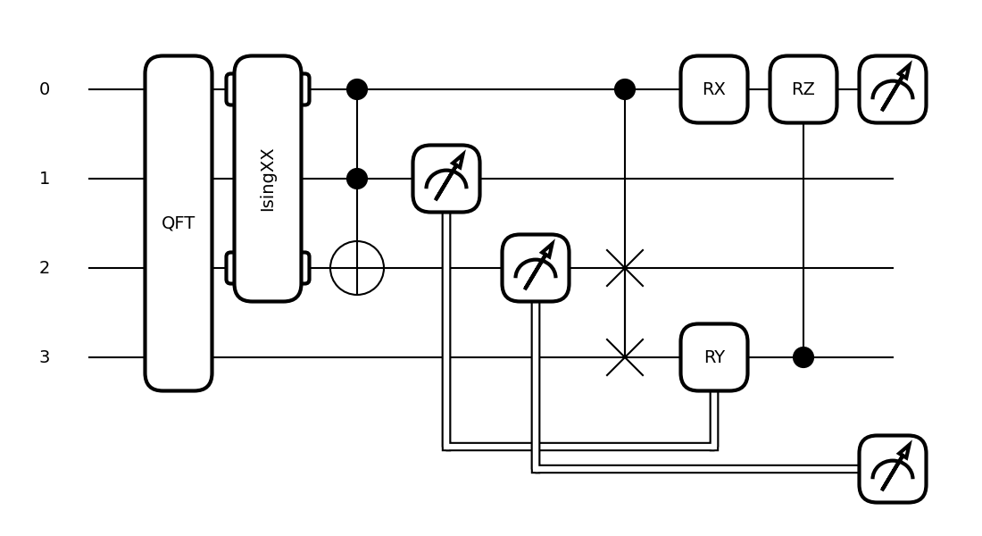
>>> print(qp.draw(circuit)(1.2345,1.2345))
0: ─╭QFT─╭IsingXX(1.23)─╭●───────────╭●─────RX(1.23)─╭RZ(1.23)─┤  <Z>
1: ─├QFT─│──────────────├●──┤↗├──────│───────────────│─────────┤
2: ─├QFT─╰IsingXX(1.23)─╰X───║───┤↗├─├SWAP───────────│─────────┤
3: ─╰QFT─────────────────────║────║──╰SWAP──RY(0.79)─╰●────────┤
                             ╚════║═════════╝
                                  ╚════════════════════════════╡  Probs[MCM]
More information, including various fine-tuning options, can be found in the drawing module.
Debugging with mid-circuit snapshots
When debugging quantum circuits run on simulators, we may want to inspect the current quantum state between gates.
Snapshot is an operator like a gate, but it saves the device state at its location in the circuit instead of manipulating the quantum state.
Currently supported devices include:
default.qubit: each snapshot saves the quantum state vectordefault.mixed: each snapshot saves the density matrix
A Snapshot can be used in a QNode like any other operation:
dev = qp.device("default.qubit", wires=2)

@qp.qnode(dev, interface=None)
def circuit():
    qp.Snapshot(measurement=qp.expval(qp.Z(0)))
    qp.Hadamard(wires=0)
    qp.Snapshot("very_important_state")
    qp.CNOT(wires=[0, 1])
    qp.Snapshot()
    return qp.expval(qp.X(0))
During normal execution, the snapshots are ignored:
>>> circuit()
0.0
However, when using the snapshots()
transform, intermediate device states will be stored and returned alongside the
results.
>>> qp.snapshots(circuit)()
{0: 1.0,
'very_important_state': array([0.707+0.j, 0.+0.j, 0.707+0.j, 0.+0.j]),
2: array([0.707+0.j, 0.+0.j, 0.+0.j, 0.707+0.j]),
'execution_results': 0.0}
All snapshots are numbered with consecutive integers, and if no tag was provided, the number of a snapshot is used as a key in the output dictionary instead.
Interactive Debugging on Simulators
PennyLane allows for more interactive debugging of quantum circuits in a programmatic
fashion using quantum breakpoints via breakpoint(). This feature is
currently supported on default.qubit and lightning.qubit devices.
Consider the following python script containing the quantum circuit with breakpoints.
dev = qp.device("default.qubit", wires=2)

@qp.qnode(dev)
def circuit(x):
    qp.breakpoint()

    qp.RX(x, wires=0)
    qp.Hadamard(wires=1)

    qp.breakpoint()

    qp.CNOT(wires=[0, 1])
    return qp.expval(qp.Z(0))

circuit(1.23)
Running the circuit above launches an interactive [pldb] prompt. Here we can
step through the circuit execution:
> /Users/your/path/to/script.py(8)circuit()
-> qp.RX(x, wires=0)
[pldb] list
  3
  4         @qp.qnode(dev)
  5         def circuit(x):
  6             qp.breakpoint()
  7
  8  ->         qp.RX(x, wires=0)
  9             qp.Hadamard(wires=1)
 10
 11             qp.breakpoint()
 12
 13             qp.CNOT(wires=[0, 1])
[pldb] next
> /Users/your/path/to/script.py(9)circuit()
-> qp.Hadamard(wires=1)
We can extract information by making measurements which do not change the state of the circuit in execution:
[pldb] qp.debug_state()
array([0.81677345+0.j        , 0.        +0.j        ,
       1.        -0.57695852j, 0.        +0.j        ])
[pldb] continue
> /Users/your/path/to/script.py(13)circuit()
-> qp.CNOT(wires=[0, 1])
[pldb] next
> /Users/your/path/to/script.py(14)circuit()
-> return qp.expval(qp.Z(0))
[pldb] list
  8             qp.RX(x, wires=0)
  9             qp.Hadamard(wires=1)
 10
 11             qp.breakpoint()
 12
 13             qp.CNOT(wires=[0, 1])
 14  ->         return qp.expval(qp.Z(0))
 15
 16         circuit(1.23)
[EOF]
We can also visualize the circuit and dynamically queue operations directly to the circuit:
[pldb] print(qp.debug_tape().draw())
0: ──RX─╭●─┤
1: ──H──╰X─┤
[pldb] qp.RZ(-4.56, 1)
RZ(-4.56, wires=[1])
[pldb] print(qp.debug_tape().draw())
0: ──RX─╭●─────┤
1: ──H──╰X──RZ─┤
See qp.debugging for more information and detailed examples.
Graph representation
PennyLane makes use of several ways to represent a quantum circuit as a Directed Acyclic Graph (DAG).
DAG of causal relations between ops
A DAG can be used to represent which operator in a circuit is causally related to another. There are two options to construct such a DAG:
The CircuitGraph class takes a list of gates or channels and hermitian observables
as well as a set of wire labels and constructs a DAG in which the Operator
instances are the nodes, and each directed edge corresponds to a wire
(or a group of wires) on which the “nodes” act subsequently.
For example, this can be used to compute the effective depth of a circuit, or to check whether two gates causally influence each other.
import pennylane as qp
from pennylane import CircuitGraph
from pennylane.workflow import construct_tape

dev = qp.device('lightning.qubit', wires=(0,1,2,3))

@qp.qnode(dev)
def circuit():
    qp.Hadamard(0)
    qp.CNOT([1, 2])
    qp.CNOT([2, 3])
    qp.CNOT([3, 1])
    return qp.expval(qp.Z(0))


circuit()
tape = construct_tape(circuit)()
ops = tape.operations
obs = tape.observables
g = CircuitGraph(ops, obs, tape.wires)
Internally, the CircuitGraph class constructs a rustworkx graph object.
>>> type(g.graph)
rustworkx.PyDiGraph
There is no edge between the Hadamard and the first CNOT, but between consecutive CNOT gates:
>>> g.has_path(ops[0], ops[1])
False
>>> g.has_path(ops[1], ops[3])
True
The Hadamard is connected to the observable, while the CNOT operators are not. The observable
does not follow the Hadamard.
>>> g.has_path(ops[0], obs[0])
True
>>> g.has_path(ops[1], obs[0])
False
>>> g.has_path(obs[0], ops[0])
False
DAG of non-commuting ops
The commutation_dag() transform can be used to produce an instance of the CommutationDAG class.
In a commutation DAG, each node represents a quantum operation, and edges represent non-commutation
between two operations.
This transform takes into account that not all operations can be moved next to each other by pairwise commutation:
>>> def circuit(x, y, z):
...     qp.RX(x, wires=0)
...     qp.RX(y, wires=0)
...     qp.CNOT(wires=[1, 2])
...     qp.RY(y, wires=1)
...     qp.Hadamard(wires=2)
...     qp.CRZ(z, wires=[2, 0])
...     qp.RY(-y, wires=1)
...     return qp.expval(qp.Z(0))
>>> dag_fn = qp.commutation_dag(circuit)
>>> dag = dag_fn(np.pi / 4, np.pi / 3, np.pi / 2)
Nodes in the commutation DAG can be accessed via the get_nodes() method, returning a list of
the form (ID, CommutationDAGNode):
>>> nodes = dag.get_nodes()
>>> nodes
NodeDataView({0: <pennylane.transforms.commutation_dag.CommutationDAGNode object at 0x7f461c4bb580>, ...}, data='node')
Specific nodes in the commutation DAG can be accessed via the get_node() method:
>>> second_node = dag.get_node(2)
>>> second_node
<pennylane.transforms.commutation_dag.CommutationDAGNode object at 0x136f8c4c0>
>>> second_node.op
CNOT(wires=[1, 2])
>>> second_node.successors
[3, 4, 5, 6]
>>> second_node.predecessors
[]